Control Data and Analyses
The data used in the GCP are from well designed random sources, and calibrations show near theoretical performance, allowing first order statistical comparisons against theoretical expectations. As physical devices, of course, they cannot literally match theory, so for detailed investigations and fully robust statistics, the data must be normalized using empirical parameter estimates.
In addition, because the effects are small and statistical, it is essential to understand and quantify the differences between theoretical and empirical data. We develop control
conditions or data by applying the analytical procedures to data that are not hypothesized to show any effect, as compared with the prespecified global events
that we assess in the formal series of hypothesis tests. Using resampling of unused actual data or random simulations, we can generate the appropriate control distribution against which the formal statistics can be compared.
The implication of the analyses is straightforward: Both statistical and exhaustive sampling show that while the database does of course contain spikes
when there are no identified global events,
they are in the proportion and magnitude expected from chance fluctuation. This is in contrast to the excess of spikes
found in the GCP series of event-based hypothesis tests.
Statistical Resampling
A powerful and general way to obtain an empirical control distribution is by resampling. This is a process that takes randomly chosen samples of the actual data, and subjects them to the analysis used for the formal data segments. This is repeated many times, to accumulate a sampling distribution from which empirical estimates are drawn for the mean, variance, and other statistics of interest.
From Peter Bancel's notes:
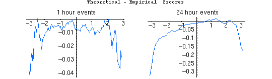
The following figures show the result of this procedure for the standard analysis, the Stouffer Z². The plots show the difference between the theoretical and empirical zscores (vertical axis) for generalized events of 1 hour duration and also of 24 hour duration (horizontal axis).
The normalized data are used to get the chisquare value for an event. The theoretical value of Z assumes Chisquare statistics for the event. This is what we normally do. The empirical value of Z estimates the p-value of the Chisquare statistic by resampling (with replacement) 1 (or 24) hour segments of the database to construct a Cumulative Distribution Function (CDF). That in turn gives an empirical p-value for a given Chisqare value, which is then converted to a zscore. A negative value of the theoretical — empirical difference means the theoretical determination understates the zscore relative to the empirical value.
The plots shown below were constructed from the results of resampling 100,000 times. The differences are generally < .01 which is very small. There is a weak trend of underestimation by the theoretical value. This is probably due to the fact that the actual Z² database has a negative trend. The noise in the 2 cases is about the same. The scales of the plots are different so the 24-hr duration plot looks smoother. There may be something to understand in the tails and drop-off of theo/empr diffs at increasing Z. Generally, it indicates that the empirical distribution (whether 1 hr or 24 hr events) is broader than the theoretical case.
This is a preliminary result (Nov 30 2005) and there remain some questions to check, for example, implications of sampling with replacement in this context. Nevertheless, the bottom line is that the theoretical and empirical zscores agree well. They yield corresponding p-values that are the same to the third or fourth decimal place.
Exhaustive Sampling
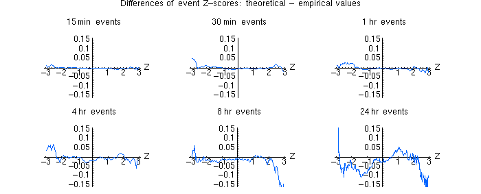
A slightly different look at the determination of empirical zscores is shown in the next plots. From Peter's description:
In this approach I use the full database from Oct 1, 1998 through Nov 12, 2005 to construct a CDF. Because the database is large, it is possible to use a full population assessment, rather than a statistical sampling approach. The results are of course similar using both methods.
I look at events
of 15, 30 minutes and 1,4,8,24 hours and compare the range of zscores using the Chisqare distribution and the empirical distribution.
Note that the empirical zscores are calculated using consecutive sections of the database, rather than a random sampling of trials. This is important because systematic drifts or autocorrelations could be lost by sampling, since the sampling would destroy the ordering of the data. The CDF is thus the distribution of zscores obtained by blocking the data into 1 hour (or 15 minute or whatever) blocks and calculating all the Z scores for the blocks. For 1 day events this gives about 2600 pts in the CDF. That means the approximation is poor as we approach z=3. The 1-hour events
make a CDF with 2600*24=62,400 pts. This gives pretty good estimations of Z out to z=3.
We don't gain by sampling more than the full database, so the database size/event size limits our z-range... This is why it's noisier for longer events.
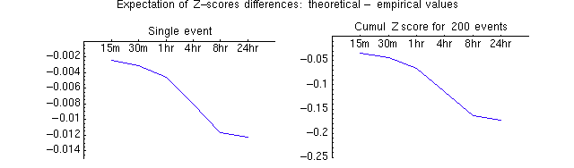
A second plot shows what we expect for a difference in z based on the 2 methods of determination. This takes into account that there are few events with large z-scores. I also show how the difference in the two methods pans out for 200 hypothetical events (of the same length). This gives a feel the importance of the difference between using theoretical and empirical z's
Note: For a cumululative Z=4 on 200 events. The 95% confidence interval (CI) is about {3.4,4.6}. The expected difference we would calculate using empirical values for event Z's would give a cumulative result of about 4.15. That is well within the CI. This means the two methods agree well.