Dean Radin
Institute of Noetic Sciences
Based on an analysis of 2.5 months of GCP data, I conclude that a statistical anomaly in this database was associated with the date, time and general location of the terrorist attacks of September 11, 2001. Of more pragmatic importance, there is evidence that the statistical anomalies began to appear about two hours before the actual events unfolded. With a much larger RNG network, distributed uniformly around the world, and with the application of more sophisticated analyses, the GCP may prove to be useful in predicting future events with similar massive impact.
Data analysis procedure
exclude raw egg values < 65 or > 135 (i.e., |z| > 4.9, probably bad data)
use resulting mean & sd to calculate z score per egg, per day
calculate z-squared per egg
sum up all z-squares across eggs, per day, keeping track of the number of eggs
create 5-minute consolidations of the per-second data, as sums of z-squares
analyze data using 6 hour sliding window
calculate z score equivalent for the resulting chi-squares & df
calculate odds associated with the z scores
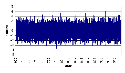
Figure
1. z scores of 5-minute summaries, across all eggs, for June 30 - September
18, 2001.
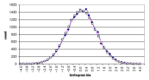
Figure
2. Histogram of z scores in Figure 1 (in black) and expected normal curve
(in red). This shows that overall the eggs are well behaved, with a slight
positive skew. The theoretical mean for the z score is 0; the observed
mean is z = -0.0002. The theoretical standard deviation is 1, the actual
sd = 0.9972. The Stouffer Z for the observed mean shift is z = -0.031.
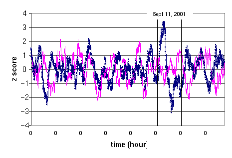
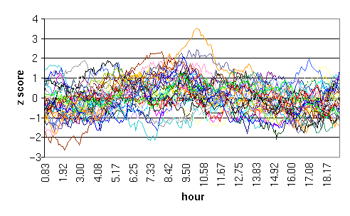
Figure
5. This shows observed z scores (in blue, 6 hour sliding window, September
3 to 13) vs. similar scores (in pink) using pseudorandomly generated data.
This confirms that the analytical method is not introducing artifacts into
the results. The "0" on the x-axis indicates the beginning of a day boundary.
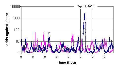
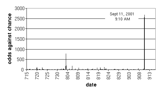
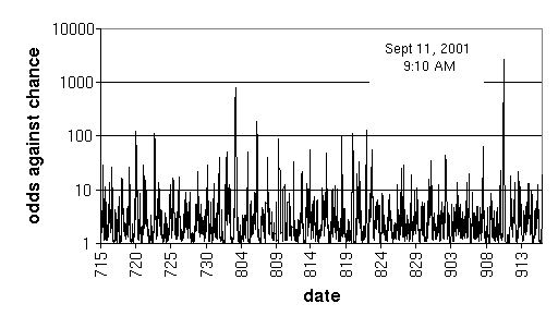
Figure
6. This shows the odds associated with the z scores in Figure 5, using
a log scale.
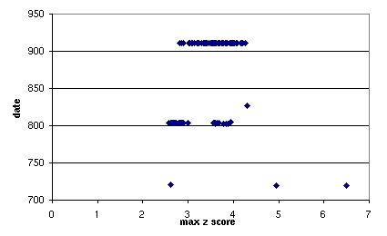
Figure
7. This shows the dates associated with maximum z scores obtained after
applying sliding windows ranging from 5 minutes to 12 hours in length,
in 5 minute increments (a total of 144 windows), to all data from July
15 - September 16. The date where the majority (60%) of the maximum z scores
occurs is September 11. This confirms that the spike observed on September
11 is not especially sensitive to the choice of specific window lengths.
The second largest cluster of maximum z scores occurs on August 4, which
is also the second largest spike in Figure 3.
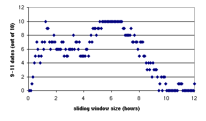
Figure
8. This shows the number of times that the date of September 11 appears
in the top 10 maximum z scores, after applying the 144 different window
lengths. We see that the majority of maximum z scores appears in window
lengths ranging from 5.2 to 6.8 hours. This suggests that the length of
the "event" on September 11 may be in this range.
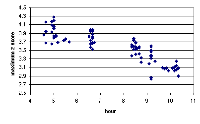
Figure
9. This shows the time of day associated with sliding windows that resulted
in maximum z scores observed on September 11. The clustering of times suggests
that the "event" may have had three especially meaningful moments: around
5 AM, 6:30 AM, and 8 -10 AM.
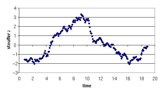
Figure
10. This shows a composite z score for September 11 across all 36 available
eggs, using a 6-hour sliding window. The peak is at 9:10 AM. This plot
is essentially a high-resolution version of the z scores shown in Figure
5, centered on September 11.
|
Egg
|
Type
|
Host
|
Category
|
Hemisphere
|
|
111
|
Auckland | New Zealand | Australia | East |
|
161
|
Sydney | Australia | Australia | East |
|
1024
|
Auckland | New Zealand | Australia | East |
|
37
|
Neuchâtel | Switzerland | Europe | East |
|
101
|
Edinburgh | Scotland | Europe | East |
|
105
|
Paris | France | Europe | East |
|
107
|
Freiburg | Germany | Europe | East |
|
112
|
Neuchâtel | Switzerland | Europe | East |
|
116
|
Wien | Austria | Europe | East |
|
134
|
Malmö | Sweden | Europe | East |
|
142
|
Søborg | Denmark | Europe | East |
|
1022
|
Braunschweig | Germany | Europe | East |
|
2006
|
England | England | Europe | East |
|
2173
|
Toulouse | France | Europe | East |
|
114
|
Madras | India | MidEast | East |
|
119
|
Grahamstown | South Africa | MidEast | East |
|
1026
|
Bangalore | India | MidEast | East |
|
2225
|
Sheva | Israel | MidEast | East |
|
108
|
Sao | Brazil | South Am | West |
|
1013
|
Mogi | Brazil | South Am | West |
|
1
|
NJ | USA | USA | West |
|
28
|
NJ | USA | USA | West |
|
34
|
NJ | USA | USA | West |
|
106
|
NY | USA | USA | West |
|
110
|
CO | USA | USA | West |
|
115
|
Alberta | Canada | USA | West |
|
118
|
CA | USA | USA | West |
|
226
|
Ontario | Canada | USA | West |
|
1005
|
CA | USA | USA | West |
|
1021
|
CA | USA | USA | West |
|
1029
|
NC | USA | USA | West |
|
1223
|
NC | USA | USA | West |
|
2000
|
WI | USA | USA | West |
|
2001
|
CA | USA | USA | West |
|
2002
|
TX | USA | USA | West |
|
2222
|
MI | USA | USA | West |
Table
1. This lists the egg numbers and their associated locations in terms of
state or region, country, continent (roughly), and hemisphere.
|
Category
|
z(9:10
AM)
|
|
West
Hemi
|
3.14
|
|
East
Hemi
|
1.57
|
Table
2. Analysis of 6-hour windowed Stouffer Z scores associated with 9:10 AM,
September 11, by combining all eggs within each hemisphere. This suggests
that a larger effect "occurred" in the Western hemisphere.
|
Category
|
Num
|
z(9:10
AM)
|
|
Australia
|
3
|
1.12
|
|
Europe
|
11
|
0.34
|
|
MidEast
|
4
|
1.80
|
|
South
Am
|
2
|
2.15
|
|
North
Am
|
16
|
2.57
|
Table
3. Analysis of 6-hour windowed Stouffer Z scores at 9:10 AM, by country,
possibly suggesting that the primary "effect" took place in Northern America.
|
Region
|
Num
|
Comp
Peak
|
|
East
|
7
|
3.0
|
|
Middle
|
5
|
0.9
|
|
West
|
4
|
0.2
|
Table
4. Analysis of North American eggs, suggesting that the primary "effect"
was in the East coast.
| Date |
9/11/2001
|
||||
| Time | 6 to 10 am |
|
|||
| Hemisphere | Western | ||||
| General area | North America | ||||
| Location | East Coast | ||||
Table
5. Summary: Through analysis of 144 sliding windows, from 5 minutes to
12 hours, in 5 minute increments, we find that over a period of 2.5 months,
one date is primarily associated with a statistical anomaly: September
11, 2001. On this date, the time range appearing most often is 6 AM to
10 AM, with a peak at 9:10 AM. The Western hemisphere appears to be responsible
for the majority of the statistical anomaly, especially North America,
and in particular the East Coast.